Learning Binary Representations of Semantic Embeddings
Reference implementation is currently private and not available. A cleaned version will be published soon.
Last updated: January 17, 2026. Experimental results section coming soon.
Intro
This blog post introduces bRose (Binary representation of semantic embeddings), a method for converting CLIP1 (or other contrastively learned) embeddings into binary representations. The approach is motivated by potential benefits in memory usage, search speed, and interpretability, though the practical value of these trade-offs remains an open question.
The method is based on a geometric observation: binary vectors correspond to corners of the unit hypercube. This leads to an optimization problem that can be solved through partial sum maximization.
The work began as an exploration of binary representation learning. How would one train such a system? How well does it work? What limitations does it have? This post describes the approach and examines these questions.
Prerequisites
It is assumed that the reader is familiar with CLIP1 (and related methods like CLOOB2, SigLIP3, MobileCLIP4, MobileCLIP25, and DFN-CLIP6)
In the following, the term “CLIP1” is used as a stand-in for other contrastive methods (CLIP, CLOOB, SigLIP, MobileCLIP, MobileCLIP2, DFN-CLIP, etc.). “CLIP1” is chosen for its familiarity.
bRose
The Idea
First, we make a trivial observation: that binary vectors are vertices of the unit hypercube. Let’s assume we are in $R^3$, then we have (unsurprisingly) the following vertices (excluding the origin):
\[\begin{equation} \mathcal{B}_3 := \{0,1\}^3 \setminus \mathbf{0} = \left\{ \begin{bmatrix} 1 \\ 0 \\ 0 \end{bmatrix}, \begin{bmatrix} 0 \\ 1 \\ 0 \end{bmatrix}, \begin{bmatrix} 0 \\ 0 \\ 1 \end{bmatrix}, \begin{bmatrix} 1 \\ 1 \\ 0 \end{bmatrix}, \begin{bmatrix} 1 \\ 0 \\ 1 \end{bmatrix}, \begin{bmatrix} 0 \\ 1 \\ 1 \end{bmatrix}, \begin{bmatrix} 1 \\ 1 \\ 1 \end{bmatrix} \right\} \end{equation}\]
The idea consists of two parts:
- a) learn to map CLIP embeddings into the unit hypercube via small FCNs and
- b) project the new embeddings onto the closest vectors in $\mathcal{B}_D$
Here only b) is somewhat challenging. There is a surprisingly simple solution, however. But more on that later. First, we will start with a).
a) Mapping Embeddings into the Unit Hypercube
The first task is to learn embeddings that lie somewhere inside the unit hypercube. For this we can use any contrastive loss (for the experiments described we use the usual CLIP1 loss). Formally, we want two properties for a resulting embedding $\mathbf{v}$:
\[\begin{equation} \label{eq:positive-embs} \mathbf{v} \in [0, 1]^D \end{equation}\]and
\[\begin{equation} \label{eq:unit_norm} ||\mathbf{v}|| = 1 \end{equation}\]In order to achieve (\ref{eq:positive-embs}) we can learn a small FCN $f_{\mu}$ for each mode $\mu$. By using the softplus activation function as output activation we ensure positive outputs:
\[\begin{equation} \label{eq:softplus} \log(1 + e^{x}) \end{equation}\]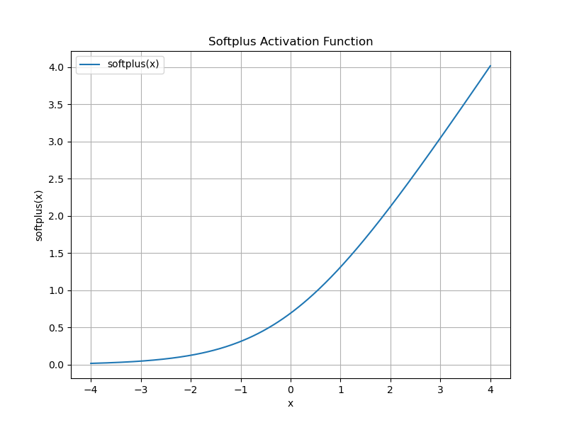
This has, of course, the consequence that the inner product of two new embeddings $\mathbf{x}$ and $\mathbf{y}$ is now positive as well: $\mathbf{x}^T \mathbf{y} \in [0, 1]$. Thus an inner product of $0$ indicates maximal dissimilarity.
So far so good. But given an output embedding, how do we assign a binary vector?
b) Finding the Right Projection
Let’s assume we have trained our FCNs to our satisfaction and apply them to some data. We receive an embedding vector $\mathbf{v} \in [0, 1]^D$ and need to assign it to the “most similar” binary vector. We will do the following:
- generate vectors of norm 1 which represent the binary vectors (referred to as proxy $\mathcal{U}_D$ for $\mathcal{B}_D$)
- assign $\mathbf{v}$ to the closest $\mathbf{u} \in \mathcal{U}_D$ in terms of some distance/similarity measure.
A Proxy for $\mathcal{B}_D$
A useful proxy can be generated by normalizing all vectors in $\mathcal{B}_D$. This will yield the following set:
\[\begin{equation} \mathcal{U}_D := \left\{ { \frac{1}{ \sqrt{\mathbf{b}^T \mathbf{1}}} \mathbf{b} \mid \mathbf{b} \in \mathcal{B}_D} \right\} \end{equation}\]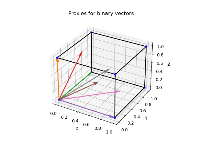
Here, $\mathbf{b}^T \mathbf{1}$ counts the number of non-zero entries in $\mathbf{b}$. And since a binary vector with $n$ non-zero entries has length $\sqrt{n}$ we just need to divide $\mathbf{b}$ by $\sqrt{\mathbf{b}^T \mathbf{1}}$ to receive a vector with norm 1.
The optimization problem
For a given embedding $\mathbf{v} \in [0, 1]^D$ we now want to assign the closest vector in $\mathcal{U}_D$. Since all involved vectors are of unit norm it does not matter if we write the optimization problem as minimizing the difference in squared L2 norm or maximizing cosine similarity:
\[\begin{equation} \label{eq:optim} \underset{ \mathbf{u} \in \mathcal{U}_D}{\operatorname{argmin}} || \mathbf{v} - \mathbf{u} ||^2, \end{equation}\]where expanding the squared norm results in
\[\begin{equation} \label{eq:sq_norm} || \mathbf{v} - \mathbf{u} ||^2 = ||\mathbf{v}||^2 - 2 \mathbf{v}^T\mathbf{u} + ||\mathbf{u}||^2 = ~ 2 - 2 ~\mathbf{v}^T\mathbf{u}, \end{equation}\]and thus
\[\begin{equation} \label{eq:optim_cos } \underset{ \mathbf{u} \in \mathcal{U}_D}{\operatorname{argmin}} || \mathbf{v} - \mathbf{u} ||^2 = \underset{ \mathbf{u} \in \mathcal{U}_D}{\operatorname{argmax}} ~ \mathbf{v}^T\mathbf{u}. \end{equation}\]If we rewrite the problem in terms of $\mathbf{b}$ we get:
\[\begin{equation} \label{eq:optim_step1} \underset{ \mathbf{b} \in \mathcal{B}_D}{\operatorname{argmax}} ~ \frac{1}{\sqrt{\mathbf{b}^T \mathbf{1}}} ~ \mathbf{v}^T\mathbf{b}. \end{equation}\]Remember that $\mathbf{b}$ is binary. So (\ref{eq:optim_step1}) tells us that a solution to the optimization problem will
- select as few as possible entries of $\mathbf{v}$ since $ \frac{1}{\sqrt{\mathbf{b}^T \mathbf{1}}}$ should be as large as possible (sparsity!)
- select the largest entries of $\mathbf{v}$
Fortunately, the gods of machine learning are kind to us and we can simply write down a function that helps us find this optimum.
Finding the solution: a partial sum for complete optimization
But first, notation: we take inspiration from programming languages, denote the function that returns the indices of the sorted (descending) entries of a vector as “$\text{argsort}$” and introduce the indexing operator $[\cdot]$. We apply this notation to get the following:
\[\begin{equation} \label{eq:argsort} \mathbf{p} = \text{argsort}(\mathbf{v}) \end{equation}\]and denote the sorted vector as
\[\begin{equation} \label{eq:sort } \mathbf{v}[\mathbf{p}]. \end{equation}\]Now, for $0 < i < j \leq D $ we have:
\[\begin{equation} \label{eq:sorted } \mathbf{v}[\mathbf{p}]_i ~ \geq ~ \mathbf{v}[\mathbf{p}]_j ~ \geq ~ \mathbf{0}. \end{equation}\]We define a function such that finding its maximum also yields the optimal binary vector. This function is the following partial sum:
\[\begin{equation} \label{eq:partial_sum} \mathcal{S}(K; \mathbf{v}) = \frac{1}{\sqrt{K}} \sum_{k=1}^K \mathbf{v}[\mathbf{p}]_k. \end{equation}\]If we find the $K^\ast$ that optimizes this sum we are done: these $K^\ast$ entries of the index vector $\mathbf{p}$ tell us exactly which entries of the binary vector need to be one (the rest is zero). Formulated differently, these $K^\ast$ entries of $\mathbf{p}$ contain the indices of the optimal binary vector $\mathbf{b}^*$ that are $1$:
\[\begin{equation} \label{eq:optimum} \mathbf{b}^*_{\mathbf{p}[1]}, \ldots, \mathbf{b}^*_{\mathbf{p}[K^*]} = 1 \quad \text{and} \quad {\mathbf{b}^*}^T \mathbf{1} = K^*; \quad \mathbf{b}^* \in \mathcal{B} \end{equation}\]Solution to (\ref{eq:optim_step1})
- In order to find the optimum we calculate all partial sums and select $K^* = \underset{K}{\operatorname{argmax}} \mathcal{S}(K)$
- Given $K^*$ The optimal binary vector $\mathbf{b}^* \in \mathcal{B_D}$ is the the one described in (\ref{eq:optimum})
Let’s plot $\mathcal{S}(K)$ for some learned embeddings after the softplus, normalized to 1:
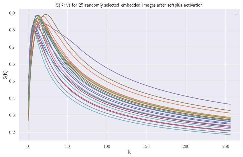
This plot would suggest that we do not need to calculate all partial sums up until $D$, but only until we have found a $K$ such that $\mathcal{S}(K) > \mathcal{S}(K+1)$. Unfortunately we can find vectors $\hat{\mathbf{v}}$ such that $\mathcal{S}(K; \hat{\mathbf{v}})$ has a minimum as extremum. More on that in the Appendix.
Extension to Ternary Embeddings
The same algorithm extends to ternary representations (values in {-1, 0, +1}) by applying the S-maximizer to the absolute values of signed embeddings and then reattaching the original signs. A convenient storage format is “ternary-as-binary”: for a ternary vector $\mathbf{t} \in {-1,0,1}^D$, store
Since ternary embeddings are signed, we do not need a softplus output activation in this mode.
\[\begin{equation} \mathbf{t}_{\text{bin}} = [\mathbf{t}^+ ~|~ \mathbf{t}^-], \quad \mathbf{t}^+_i = \mathbb{1}[t_i = +1], \; \mathbf{t}^-_i = \mathbb{1}[t_i = -1]. \end{equation}\]This keeps the representation binary while preserving sign information, and it lets us reuse the projection machinery with minimal changes.
Encouraging Better Projections During Training
Alignment
While the projection method finds the optimal binary vector for any given embedding, we can encourage the learned embeddings to be closer to their eventual binary projections during training. An alignment loss helps by pulling embeddings toward hypercube vertices:
\[\begin{equation} \mathcal{L}_{\text{align}}(\mathbf{x}, \mathbf{y}) = \frac{1}{2}\left( \|\mathbf{x} - \hat{\mathbf{b}}^*\|^2 + \|\mathbf{y} - \hat{\mathbf{b}}^*\|^2 \right) \end{equation}\]where $\hat{\mathbf{b}}^*$ is the normalized binary projection of whichever embedding ($\mathbf{x}$ or $\mathbf{y}$) is already better aligned to its own binary representation. The intuition is that if one embedding is already closer to being binary, both embeddings should move toward that target.
Ternary alignment loss
For signed embeddings, we use the same idea but align against ternary projections. Let $\tau(\mathbf{x})$ be the ternary projection of $\mathbf{x}$ (converted back to ${-1,0,1}^D$ and normalized). We pick the better-aligned ternary target between $\tau(\mathbf{x})$ and $\tau(\mathbf{y})$ and pull both embeddings toward it:
\[\begin{equation} \mathcal{L}_{\text{align}}^{\text{ternary}}(\mathbf{x}, \mathbf{y}) = \frac{1}{2}\left( \|\hat{\mathbf{x}} - \hat{\mathbf{t}}^*\|^2 + \|\hat{\mathbf{y}} - \hat{\mathbf{t}}^*\|^2 \right). \end{equation}\]Uniformity on the hypersphere
While alignment pulls embeddings toward binary vertices, it is also important to keep the representation uniformly spread over the unit hypersphere to avoid collapse and to preserve semantic separation before binarization. Wang and Isola emphasize this alignment-uniformity trade-off in contrastive learning7. A common uniformity term is:
\[\begin{equation} \mathcal{L}_{\text{uniform}} = \log \mathbb{E}_{\mathbf{x}, \mathbf{y}} \left[\exp(-2 \|\mathbf{x} - \mathbf{y}\|^2)\right] \end{equation}\]Minimizing this term discourages high-density regions on the sphere, which can make the eventual binary projections more balanced and stable.
The total training loss can then be written as:
\[\begin{equation} \mathcal{L}_{\text{total}} = \mathcal{L}_{\text{contrastive}} + \lambda_{\text{align}} \mathcal{L}_{\text{align}} + \lambda_{\text{uniform}} \mathcal{L}_{\text{uniform}}, \end{equation}\]using $\mathcal{L}_{\text{align}}^{\text{ternary}}$ in ternary mode.
Implementation
A PyTorch reference implementation is available in the linked repository. The core algorithm implements the partial sum maximization described above. See Appendix B for the complete code.
Comparing binary representations
After calculating binary representations we of course want to compare them — we need a similarity function. The obvious choice is the Jaccard Index (or IoU):
\[\begin{equation} \mathcal{J}(\mathbf{x}, \mathbf{y}) = \frac{ \mathbf{x}^T \mathbf{y}}{ \mathbf{x}^T \mathbf{1} + \mathbf{y}^T \mathbf{1} - \mathbf{x}^T \mathbf{y}}; \quad \mathbf{x}, \mathbf{y} \in \mathcal{B}_D. \end{equation}\]$\mathcal{J}(\mathbf{x}, \mathbf{y}) = 1$ if the exact same entries are active in both $\mathbf{x}$ and $\mathbf{y}$ and $0$ if no entries match. Importantly, the similarity is downweighted if one of the binary representations has many more active entries than the other.
Ternary Jaccard similarity
| For ternary-as-binary vectors $\mathbf{q} = [\mathbf{q}^+ | \mathbf{q}^-]$ and $\mathbf{d} = [\mathbf{d}^+ | \mathbf{d}^-]$, a signed Jaccard-style score is: |
The numerator counts agreements minus disagreements, and the denominator is the union of all active positions (ignoring sign). The score lies in $[-1, +1]$.
Note (similarity search): In practice, compute this via bitwise popcount on masks: agreements from $(\mathbf{q}^+ \land \mathbf{d}^+) + (\mathbf{q}^- \land \mathbf{d}^-)$, disagreements from $(\mathbf{q}^+ \land \mathbf{d}^-) + (\mathbf{q}^- \land \mathbf{d}^+)$, and the union from $(\mathbf{q}^+ \lor \mathbf{q}^-) \lor (\mathbf{d}^+ \lor \mathbf{d}^-)$. This form supports early pruning: if the running numerator upper bound drops below $0$, the final similarity cannot become positive.
Why Is the Hamming Distance Not Used?
The Hamming distance counts the different entries between two binary vectors (in our case). It would be simple to change the Hamming distance $h(\cdot)$ to a Hamming similarity $h_s(\cdot) = 1 - h(\cdot)/D$. To see why the Hamming distance (or similarity) is not suitable for our case, let’s consider two vectors:
\[\begin{equation} \label{eq:hamming-vec} \mathbf{v}_1 = [1, 0, 0, 0], \quad \mathbf{v}_2 = [0, 0, 0, 1] \end{equation}\]It is clear that for the Jaccard index we have $\mathcal{J}(\mathbf{v}_1, \mathbf{v}_2) = 0$. This is what we would expect, since there are two completely different “concepts” active (e.g. one could be dog, the other car). However, the Hamming distance would be $h(\mathbf{v}_1, \mathbf{v}_2) = 2$ and the Hamming similarity would be $h_s(\mathbf{v}_1, \mathbf{v}_2) = 0.5$ since half of the entries are the same. The larger $D$ the more severe this issue becomes. For $D = 256$, in this case we would get a Hamming similarity of $\approx 0.99$ which is clearly not what we want.
Acknowledgements
Many thanks to Rahul Siripurapu for providing valuable feedback!
Appendix
A) Examples of $S(K)$ with a Minimum as Extremum
When first deriving the method, I believed that it might be enough to find a $K$ such that $\mathcal{S}(K) > \mathcal{S}(K+1)$ (except for the case $K^\ast = D$). For some readers it might be obvious that this is not the case — it took some time for me. In the end I tried to find counterexamples. The following counterexample is a $\hat{\mathbf{v}}$ such that $\mathcal{S}(K; \hat{\mathbf{v}})$ has a minimum as extremum.
We construct a $\hat{\mathbf{v}}$ such that for a $\alpha \in [0, 1]$ we have that $(100 \cdot \alpha) \%$ of the mass is distributed to the first entry and $(100 \cdot [1-\alpha]) \%$ is distributed uniformly to the rest of the entries. We set $\alpha = 0.5$ and construct $\hat{\mathbf{v}}$:
\[\label{eq:counter-example-1} \sum_{i=1}^D \hat{\mathbf{v}}_i^2 = 1 \iff \hat{\mathbf{v}}_1^2 = 1 - \sum_{i=2}^D \hat{\mathbf{v}}_i^2\]and since for all $ i, j \geq 2$ our entries are equal $\hat{\mathbf{v}}_i = \hat{\mathbf{v}}_j$, we can calculate their value as
\[\label{eq:counter-example-2} \hat{\mathbf{v}}_1^2 = 1 - \sum_{i=2}^D \hat{\mathbf{v}}_i^2 = 1 - (D-1) \hat{\mathbf{v}}_2^2 \implies\] \[\label{eq:counter-example-3} \sqrt{\frac{1 - \hat{\mathbf{v}}_1^2}{D-1}} = \hat{\mathbf{v}}_2\]where $\hat{\mathbf{v}}_2$ represents all $\hat{\mathbf{v}}_i$ for $i \geq 2$. In order to distribute $50 \%$ of the mass to the first entry and equally to the rest, we have to set $\hat{\mathbf{v}}_1^2 = 0.5$ and $\hat{\mathbf{v}}_2^2 = 0.00196078431372549$ which results in $\hat{\mathbf{v}}_1 = 0.7071067811865476$ and $\hat{\mathbf{v}}_2 = 0.04428074427700476$. If we plot $S(K;\hat{\mathbf{v}})$ we get the following plot which clearly serves as a counterexample to my initial assumption:
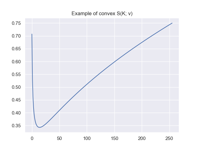
Unfortunately this means that we need to check for the argmax up to $K = D$.
B) Reference Implementation
Below is the PyTorch implementation of the binary projection algorithm using vectorized operations:
1
2
3
4
5
6
7
8
9
10
11
12
13
14
15
16
17
18
19
20
21
22
23
24
25
26
27
28
29
30
31
32
33
34
35
36
37
38
39
40
41
42
43
import torch
from torch import vmap
import torch.nn.functional as F

def batched_s_maximizer(dim: int, device: torch.device):
    # Pre-compute scalers: 1/√1, 1/√2, ..., 1/√D for the partial sums
    scalers = 1.0 / ((torch.arange(1, dim + 1).to(device)).sqrt())

    def s_maximizer(x: torch.Tensor):
        # Sort embedding values in descending order, get permutation indices
        p = torch.argsort(x, descending=True, dim=-1)

        # Compute S(K) = (1/√K) * Σ(top K values) for all K=1..D
        # x[..., p] reorders x according to sorted indices
        s = scalers * torch.cumsum(x[..., p], dim=-1)

        # Find K that maximizes S(K)
        idx = torch.argmax(s, dim=-1)

        return idx, p

    # Return vectorized version that works on batches
    return vmap(s_maximizer)

def project_positive_vector_to_binary(v: torch.Tensor) -> torch.Tensor:
    # Normalize to unit length (required for the optimization)
    v = F.normalize(v, dim=-1)

    # Find optimal K and sorting permutation for each embedding in the batch
    bidx, bp = batched_s_maximizer(dim=v.size(-1), device=v.device)(v)

    D = v.size(-1)

    # Create range tensor [0, 1, 2, ..., D-1] with proper broadcasting shape
    rank = torch.arange(D, device=v.device).view(*([1] * (v.dim() - 1)), D)

    # Create binary mask: first bidx+1 elements are True (since we want K elements, 0-indexed)
    mask_sorted = rank <= bidx.unsqueeze(-1)

    # Apply mask to original embedding positions using scatter
    # bp contains the original indices in sorted order
    # mask_sorted determines which of the top-K positions get value 1
    return torch.zeros_like(v).scatter(-1, bp, mask_sorted.to(v.dtype))
Citation Information
If you find bRose useful and intend to use it, please cite this blog via:
1
2
3
4
5
6
@misc{Ramsauer2024,
  author = {Hubert Ramsauer},
  title = {bRose: Binary Representation of Semantic Embeddings},
  year = {2024},
  url = {https://HubiRa.github.io/posts/brace/},
}
References
A. Radford et al., Learning Transferable Visual Models From Natural Language Supervision. International Conference on Machine Learning, 2021 ↩︎ ↩︎2 ↩︎3 ↩︎4 ↩︎5
A. Fürst et al., CLOOB: Modern Hopfield Networks with InfoLOOB Outperform CLIP. Neural Information Processing Systems, 2022 ↩︎
X. Zhai et al., Sigmoid Loss for Language Image Pre-Training. International Conference on Computer Vision, 2023 ↩︎
P. Ao et al., MobileCLIP: Fast Image-Text Models through Multi-Modal Reinforced Training, arXiv preprint arXiv:2311.17049, 2023 ↩︎
Y. Liu et al., MobileCLIP2: Fast Image-Text Models through Multi-Modal Reinforced Training and Model Scaling, arXiv preprint arXiv:2508.20691, 2025 ↩︎
K. Li et al., DFN-CLIP: Data-Free Network CLIP, arXiv preprint arXiv:2309.17425, 2023 ↩︎
T. Wang and P. Isola, Understanding Contrastive Representation Learning through Alignment and Uniformity on the Hypersphere, arXiv preprint arXiv:2005.10242, 2020 ↩︎